Smoothing options prices with linear programming

Key Takeaway

• One goal of fitting: Fitting implied volatility (IV) surfaces helps smooth out the effects of market illiquidity and noise.
• The interpolation trap: Simple piece-wise linear interpolation on raw data is unusable because it overfits market noise and creates arbitrage.
• A shift in perspective: Smoothing raw prices instead of IVs allows Linear Programming to enforce arbitrage rules simply and transparently, enabling more flexible fitting.

Why we fit: Smoothing the noise of illiquidity

In an ideal world, market prices would be perfectly efficient and continuous. In reality, the options market is often affected by illiquidity, wide bid-ask spreads, and noisy data points.

To make sense of this, the standard quantitative workflow follows a specific path:

1. Compute the raw implied volatilities (IVs) from market prices.
2. Fit a surface to these IVs to smooth out the noise.
3. Price the options and manage risk using this smoothed surface.

The fitting step is the most critical. If we simply used piece-wise linear interpolation (connecting the dots) on raw market data, the result would be a “wiggly” surface that mirrors every tiny market anomaly and bid-ask bounce. This can be dangerous, as it fails to smooth out illiquidities and can lead to arbitrage opportunities.

In our previous blog posts, we explored how to address this by fitting the implied volatilities (IVs) directly. We discussed traditional parametric models like SSVI and more advanced, flexible approaches like Physics-Informed Neural Networks (PINNs). These methods are designed to force a mathematically safe shape onto the IV surface to ignore the noise and extract a clean signal.

A new perspective: Smoothing prices directly

What if we change the order of operations? Instead of forcing complex mathematical models onto the IV surface, we can apply the smoothing process directly to the raw option prices themselves.

By cleaning up the prices first, we can extract the implied volatilities only after the market noise and arbitrage opportunities have been filtered out. This subtle shift in perspective unlocks a highly efficient mathematical optimization tool: linear programming (LP).

The linear programming engine

When modeling IVs, preventing static arbitrage is a non-linear nightmare. In our previous blogs, we discussed that IVs’ non-arbitrage conditions translate into complex Partial Differential Equations (PDEs). However, if we look at raw European and American option prices, the rules that govern an arbitrage-free market arey simple linear constraints.

To guarantee our prices are free from the primary static arbitrage traps (Calendar Spread, Vertical Spread, and Butterfly), the LP framework enforces three simple rules:

• • Time value (no calendar arbitrage): Options must become more expensive as time to expiration increases.
    Constraint:
    Note that this constraint can break for deep ITM American options with high dividend yields. For American options, we are only able to protect ourselves from Vertical and Butterfly Spreads with mathematical certainty.
  • Moneyness (no vertical arbitrage): For call options, the price must decrease as the strike price increases (and vice versa for puts).
    Constraint (for calls):
    
  • Convexity (no butterfly arbitrage): The rate at which prices change between strikes must ensure convexity.
    Constraint:

Because these rules are linear, we can use a standard LP solver to minimize the error between our adjusted prices and the observed market prices. The solver acts as a mathematical smoother, pressing out the “wrinkles” of illiquidity. The result is a set of prices that are as close as possible to the market, but strictly bounded by the laws of financial logic.

For technical readers interested in the full mathematical formulation, this framework builds on the foundational work by Cohen, Reisinger, and Wang in their paper Detecting and repairing arbitrage in traded option prices.

Safely unlocking piece-wise linear interpolation

Once we have this newly smoothed grid of option prices, we can compute the IVs. Now, the final step, interpolation, becomes easy.

Earlier, we said piece-wise linear interpolation was “dangerous” and “too wiggly.” That was only true when applied to raw, noisy data. But because the LP framework has already smoothed out illiquidities and ensured the prices are free from the main static arbitrage opportunities, the resulting IV surface is inherently stable.

With the danger of overfitting eliminated, we are finally free to apply piece-wise linear interpolation to these IVs. Alternatively, LP can act as a powerful data-cleaning step prior to any fitting framework, including SSVI or neural networks.

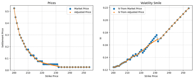
The plot below illustrates how the LP engine cleans some Out-of-the-Money (OTM) call prices for Live Cattle. By enforcing no-arbitrage constraints on the prices, the resulting Implied Volatilities become significantly smoother. This stability is what finally allows piece-wise linear interpolation to provide a precise fit (in orange) without the usual noise of raw market data (in blue).

Transparency: Knowing “why” prices move

Beyond efficiency, this framework offers a level of transparency that traditional models lack. Parametric fitting can often feel obscure – when a model price differs from the market, it’s usually just a byproduct of the model’s mathematical stiffness. There is no clear financial reason for the gap.

In contrast, the LP framework tells you exactly why a given price was adjusted. If our smoothed price differs from the market, it is specifically because the original market data was illiquid and violated a concrete arbitrage constraint. You can trace every adjustment back to a broken rule, whether it was a lack of convexity or a calendar spread violation. This makes the entire process auditable and financially grounded.

Conclusion: The best of both worlds

By shifting the smoothing process from volatilities to prices, we simplify the math while guaranteeing strict adherence to no-arbitrage rules. The LP framework acts as a filter, allowing us to safely use simple interpolation methods to achieve a robust and transparent solution to the volatility fitting problem.