The science behind safe and accurate volatility models: How Neural Networks learn financial rules

• Physics-informed Neural Networks capture market patterns while enforcing financial laws.
• Curriculum training ensures robust and stable learning.
• Transfer learning dramatically reduces training time.

In our previous blog, we explored how traditional implied volatility models struggle to balance accuracy and arbitrage-freeness. Based on this, we introduced our hybrid solution, which consists of a neural network-based model that learns how to capture fine-grained patterns in market data. At the same time, it strictly adheres to no-arbitrage constraints, delivering high accuracy without compromising financial integrity.

Here, we delve a bit deeper into the technical details of our approach and, in particular, discuss the implications of integrating financial sector knowledge into artificial intelligence (AI) processes.

The problem: Why volatility models need rules

Imagine predicting the weather with a model that’s great at forecasting precipitation but ignores the laws of physics: it might tell you it will rain when temperatures are below freezing, instead of correctly predicting snow.

Similarly, modeling implied volatility (IV) isn’t just about accuracy; it’s about respecting financial “laws” that prevent arbitrage: risk-free profits that break the market’s logic.

The three arbitrage traps to avoid are calendar spread arbitrage, vertical spread arbitrage, and butterfly arbitrage: for the details, see our previous blog.

As we saw there, traditional models either oversimplify the IV surface (missing details) or become too flexible (ignoring arbitrage rules). Let’s break down how neural networks (NNs) can solve this problem.

Understanding NNs: MLPs, loss functions, and optimization

NNs are computational models inspired by the structure and function of the human brain, designed to recognize patterns and solve complex problems by learning from data. At the core of many architectures, like ours, is the Multi-Layer Perceptron (MLP), which consists of an input layer, one or more hidden layers, and an output layer. Each layer is made up of interconnected neurons, where each connection is assigned a weight, influencing how input data is transformed as it propagates through the network.

The learning process in an MLP begins with the definition of a loss function: a mathematical function that quantifies the error between the network predictions and the actual target values. In our case, we chose the Mean Absolute Relative Error (MARE) as the loss function, since it is less sensitive to outliers than squared errors and prevents high and illiquid volatilities from dominating the loss due to its relative scaling. Optimization algorithms iteratively adjust the weights to minimize this loss. This iterative process enables the network to improve its predictions progressively, forming the backbone of modern deep learning systems.

Physics-informed Neural Networks: Teaching finance to AI

Physics-Informed Neural Networks (PINNs) constitute an innovative approach that combines traditional neural networks (MLPs) with established physical laws. Unlike standard neural networks that learn solely from data, PINNs integrate known principles that can be expressed as partial differential equations (PDEs). In this context, the network not only learns from historical data, but it also minimizes the residuals in satisfying these governing equations. The term ‘residuals’ refers to the difference between the exact mathematical conditions imposed by the PDEs and the current network predictions.

This fusion of data-driven learning and strict rule enforcement allows PINNs to achieve highly accurate predictions even when data is scarce or noisy. Fortunately, the financial “laws” that prevent arbitrage are in fact PDEs and PINNs can be used to fit IV surfaces with great accuracy while still preserving no-arbitrage constraints.

An IV surface does not allow risk-free profits from calendar spread strategies if the total implied variance is not decreasing with respect to maturity, that is,

∂ω/∂T ≥ 0, where ω = σ(k,T)² T is the total implied variance, σ(k,T) is the volatility surface, and k=log (K/F_T) is the log-moneyness with strike price K, forward price F_T  and maturity T. For what concerns vertical spread and butterfly arbitrage strategies, they are neutralized

if the Durrleman’s condition is fulfilled:

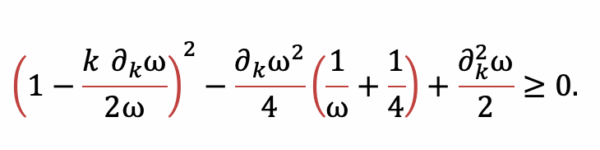
Curriculum training: Learning in stages

Training an NN to avoid arbitrage is like teaching someone to play chess: start with the basics, then add complexity.

Our three-phase approach is the following:

1. Accuracy first: The NN focuses purely on fitting market data, ignoring arbitrage rules.
2. Introduce rules gradually: Light penalties for arbitrage violations hinting the model toward safer predictions.
3. Strict enforcement: Heavy penalties ensure the final model is both accurate and rule-abiding.

This staged training prevents the NN from becoming overwhelmed and ensures stable learning. To enforce financial rules progressively, we increased the weights (λ) assigned to the PDE residuals (which measure how much the model output violates the mathematical conditions) to be minimized through an optimization algorithm.

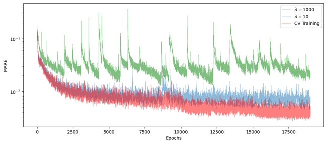
The following plot shows the behavior of the MARE loss function across 19.000 epochs of the same NN (one epoch is the one entire passing of training data through the algorithm), on a data set of NVDA American options prices from 23 October 2024. Curriculum training is in red while the others (blue and green) represent fixed-weight trains. Look how the MARE improves faster in the first case with respect to the others, suggesting a higher robustness of curriculum training compared to simple trains. Moreover, curriculum training allows one to consider extreme values of λ ,such as λ = 10000 at the last stage, while maintaining a stable train, thus ensuring that arbitrage-free conditions are easily met.

Transfer learning: Borrowing yesterday’s knowledge

Markets change daily, but they don’t reinvent the wheel overnight. Transfer learning uses prior knowledge to speed up training, and we exploited it in our model as follows:

• Day 1: Train an NN on historical IV data.
• Day 2: Instead of starting from scratch, reuse Day 1’s model as a baseline. Fine-tune it with new data.
• Day N: Fine-tune Day N-1’s model with current data.

This approach cuts training time by up to 50 percent and improves consistency, like a chef refining a recipe instead of inventing a new dish daily.

Integrating financial knowledge into NN pipelines

By embedding financial principles into AI training, we’ve created a model that’s both precise and safe. It’s not just about avoiding errors; it’s about building tools that align with how markets should behave.

For traders, this means reliable pricing. For risk managers, it’s a guardrail against hidden pitfalls. And for quants, it’s proof that innovation doesn’t have to mean complexity.